Building Metapaths by OSMNx and City2Graph¶

This notebook demonstrates how to construct a metapath on a heterogeneous graph using City2Graph.

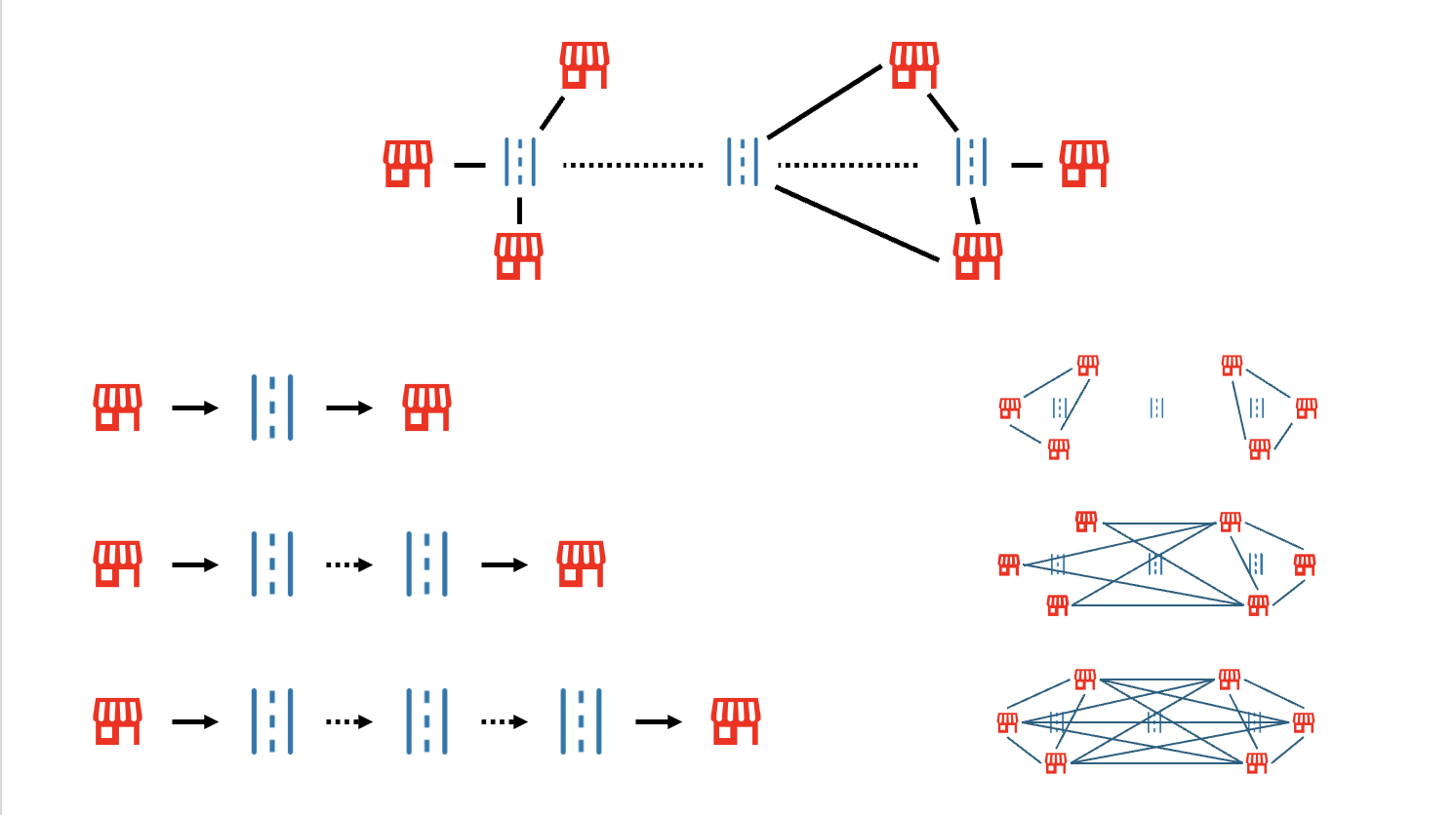
A metapath defines a composite relation between nodes in a heterogeneous graph, widely used in Graph Neural Networks (GNN).

For example, Amenity -> Segment -> Segment -> Amenity connects two amenities if they are accessible via a short walk (two street segments).

We will:

1. Fetch Data: Get the street network and amenities for Soho, London using osmnx (OpenStreetMap).
2. Construct Graph: Create a dual graph of the streets using NetworkX concepts.
3. Bridge Nodes: Connect amenities to the street network using spatial joins with GeoPandas.
4. Add Metapaths: Materialize the Amenity-Segment-Segment-Amenity relationship to densify the graph.
5. Visualization: Visualize the metapaths with an animation.
6. Add Metapaths by Weight: Connect amenities based on travel distance for weighted graph analysis.

In [1]:

import geopandas as gpd
import osmnx as ox
import pandas as pd
import matplotlib.pyplot as plt
from matplotlib.lines import Line2D
from matplotlib.animation import FuncAnimation
import city2graph as c2g

import geopandas as gpd import osmnx as ox import pandas as pd import matplotlib.pyplot as plt from matplotlib.lines import Line2D from matplotlib.animation import FuncAnimation import city2graph as c2g

0. What is a Metapath in Heterogeneous Graphs?¶

A metapath is a sequence of relations between node types in a heterogeneous graph. It describes a composite relationship between two nodes and is fundamental for capturing semantic information in Graph Neural Networks (GNN).

For example, in our city graph:

1. Amenity (e.g., a Cafe) is connected to a Street Segment (is_nearby).
2. Street Segment is connected to another Street Segment (connects_to).
3. Street Segment is connected to another Amenity (is_nearby).

This forms the metapath Amenity -> Segment -> Segment -> Amenity, representing that two amenities are within a short walking distance (2 segments) of each other. This structure allows GNNs to learn embeddings based on connectivity patterns.

1. Fetch Data from OpenStreetMap¶

We download the street network and amenities (cafes, pubs, etc.) for Soho, London. This time we use OpenStreetMap via OSMnx. While City2Graph supports a variety of data sources, it has direct compatibility to OSMnx objects (e.g. c2g.nx_to_gdf(), c2g.dual_graph(), c2g.nx_to_pyg() and many others), making it easy to integrate with existing geospatial workflows.

In [2]:

# Download and project the street network to British National Grid (EPSG:27700) for metric distances
# Data should be obtained from Only in Soho, London
G = ox.graph_from_place(
    "Soho, London",
    network_type="all",
)

street_primary_nodes, street_primary_edges = c2g.nx_to_gdf(G)
street_primary_nodes = street_primary_nodes.to_crs(epsg=27700)
street_primary_edges = street_primary_edges.to_crs(epsg=27700)

amenity_tags = ["cafe", "restaurant", "pub", "bar", "museum", "theatre", "cinema"]
amenity_candidates = ox.features_from_place(
    "Soho, London",
    tags={"amenity": amenity_tags},
).to_crs(epsg=27700)

# Download and project the street network to British National Grid (EPSG:27700) for metric distances # Data should be obtained from Only in Soho, London G = ox.graph_from_place( "Soho, London", network_type="all", ) street_primary_nodes, street_primary_edges = c2g.nx_to_gdf(G) street_primary_nodes = street_primary_nodes.to_crs(epsg=27700) street_primary_edges = street_primary_edges.to_crs(epsg=27700) amenity_tags = ["cafe", "restaurant", "pub", "bar", "museum", "theatre", "cinema"] amenity_candidates = ox.features_from_place( "Soho, London", tags={"amenity": amenity_tags}, ).to_crs(epsg=27700)

For the analysis, we clean up the amenities.

In [3]:

# Collapse complex Amenity geometries to points within the projected CRS
amenities = (
    amenity_candidates[["name", "amenity", "geometry"]]
    .copy()
    .explode(index_parts=False)
    .dropna(subset=["geometry"])
)
non_point_mask = ~amenities.geometry.geom_type.isin(["Point"])
amenities.loc[non_point_mask, "geometry"] = amenities.loc[non_point_mask, "geometry"].centroid
amenities = amenities.set_geometry("geometry")
amenities["name"] = amenities["name"].fillna(amenities["amenity"].str.title())
amenities = amenities[~amenities.geometry.is_empty]
amenities = amenities.drop_duplicates(subset="geometry").reset_index(drop=True)

# Collapse complex Amenity geometries to points within the projected CRS amenities = ( amenity_candidates[["name", "amenity", "geometry"]] .copy() .explode(index_parts=False) .dropna(subset=["geometry"]) ) non_point_mask = ~amenities.geometry.geom_type.isin(["Point"]) amenities.loc[non_point_mask, "geometry"] = amenities.loc[non_point_mask, "geometry"].centroid amenities = amenities.set_geometry("geometry") amenities["name"] = amenities["name"].fillna(amenities["amenity"].str.title()) amenities = amenities[~amenities.geometry.is_empty] amenities = amenities.drop_duplicates(subset="geometry").reset_index(drop=True)

In [4]:

# Display street network data
print("Street Primary Nodes:")
display(street_primary_nodes.head(3))
print("\nStreet Primary Edges:")
display(street_primary_edges.head(3))
print("\nAmenities:")
display(amenities.head(3))

# Display street network data print("Street Primary Nodes:") display(street_primary_nodes.head(3)) print("\nStreet Primary Edges:") display(street_primary_edges.head(3)) print("\nAmenities:") display(amenities.head(3))

Street Primary Nodes:

	y	x	street_count	geometry	highway	railway	ref
107324	51.515651	-0.132443	4	POINT (529683.159 181289.359)	NaN	NaN	NaN
107326	51.515148	-0.132727	4	POINT (529664.875 181232.921)	NaN	NaN	NaN
107328	51.514837	-0.132323	3	POINT (529693.803 181199.041)	NaN	NaN	NaN

Street Primary Edges:

			osmid	highway	maxspeed	name	oneway	reversed	length	geometry	lanes	access	width	tunnel	service
107324	12437701118	0	59207650	residential	20 mph	Soho Street	False	False	8.366709	LINESTRING (529683.159 181289.359, 529679.695 ...	NaN	NaN	NaN	NaN	NaN
	11310505522	0	395757466	footway	NaN	NaN	False	False	6.567612	LINESTRING (529683.159 181289.359, 529684.78 1...	NaN	NaN	NaN	NaN	NaN
	1694551556	0	4082521	residential	20 mph	Soho Square	True	False	74.927392	LINESTRING (529683.159 181289.359, 529706.44 1...	NaN	NaN	NaN	NaN	NaN

Amenities:

	name	amenity	geometry
0	Curzon Soho	cinema	POINT (529818.965 180959.788)
1	Pastaio	restaurant	POINT (529233.765 180972.225)
2	Yauatcha	restaurant	POINT (529498.558 181064.047)

2. Construct Dual Graph for Street Networks¶

We convert the primary street graph (intersections as nodes) to a dual graph (streets as nodes). In urban analytics, dual graphs are often better for analyzing connectivity and flow between streets, as edges represent the connections between street segments rather than physical intersections.

In [5]:

street_dual_nodes, street_dual_edges = c2g.dual_graph((street_primary_nodes, street_primary_edges))

street_dual_nodes.geometry = street_dual_nodes.geometry.centroid

street_dual_nodes, street_dual_edges = c2g.dual_graph((street_primary_nodes, street_primary_edges)) street_dual_nodes.geometry = street_dual_nodes.geometry.centroid

In [6]:

# Display dual graph data
print("Street Dual Nodes (Segments):")
display(street_dual_nodes.head(3))
print("\nStreet Dual Edges (Connections):")
display(street_dual_edges.head(3))

# Display dual graph data print("Street Dual Nodes (Segments):") display(street_dual_nodes.head(3)) print("\nStreet Dual Edges (Connections):") display(street_dual_edges.head(3))

Street Dual Nodes (Segments):

			osmid	highway	maxspeed	name	oneway	reversed	length	geometry	lanes	access	width	tunnel	service
107324	12437701118	0	59207650	residential	20 mph	Soho Street	False	False	8.366709	POINT (529681.427 181293.171)	NaN	NaN	NaN	NaN	NaN
	11310505522	0	395757466	footway	NaN	NaN	False	False	6.567612	POINT (529683.97 181286.175)	NaN	NaN	NaN	NaN	NaN
	1694551556	0	4082521	residential	20 mph	Soho Square	True	False	74.927392	POINT (529714.059 181289.894)	NaN	NaN	NaN	NaN	NaN

Street Dual Edges (Connections):

		geometry
from_edge_id	to_edge_id
(10693880886, 10693880887, 0)	(10693880886, 11815774945, 0)	LINESTRING (529790.105 181134.445, 529782.217 ...
	(10693880886, 12437444593, 0)	LINESTRING (529790.105 181134.445, 529809.944 ...
	(10693880887, 10693880886, 0)	LINESTRING (529790.105 181134.445, 529790.105 ...

In [7]:

c2g.plot_graph(nodes=street_primary_nodes, 
               edges=street_primary_edges)

c2g.plot_graph(nodes=street_primary_nodes, edges=street_primary_edges)

In [8]:

c2g.plot_graph(nodes=street_dual_nodes, 
               edges=street_dual_edges)

c2g.plot_graph(nodes=street_dual_nodes, edges=street_dual_edges)

3. Bridge Nodes (Connect Amenities)¶

We attach amenities to their nearest street segment (dual node) using bridge_nodes. This creates a heterogeneous graph with two node types: amenity and segment.

In [9]:

nodes_dict = {
    "amenity": amenities,
    "segment": street_dual_nodes
}

edges_dict = {
    ("segment", "connects_to", "segment"): street_dual_edges
}

# Connect amenities to segments
# bridge_nodes returns the node dictionary and a new dictionary of proximity edges
_, bridged_edges = c2g.bridge_nodes(
    nodes_dict=nodes_dict,
    proximity_method="knn",
    source_node_types=["amenity"],
    target_node_types=["segment"],
    k=1  # Connect to the single nearest segment
)

# Add the street network edges to the edges dictionary
edges_dict.update(bridged_edges)

nodes_dict = { "amenity": amenities, "segment": street_dual_nodes } edges_dict = { ("segment", "connects_to", "segment"): street_dual_edges } # Connect amenities to segments # bridge_nodes returns the node dictionary and a new dictionary of proximity edges _, bridged_edges = c2g.bridge_nodes( nodes_dict=nodes_dict, proximity_method="knn", source_node_types=["amenity"], target_node_types=["segment"], k=1 # Connect to the single nearest segment ) # Add the street network edges to the edges dictionary edges_dict.update(bridged_edges)

In [10]:

bridged_edges.keys()

bridged_edges.keys()

Out[10]:

dict_keys([('amenity', 'is_nearby', 'segment')])

In [11]:

bridged_edges[('amenity', 'is_nearby', 'segment')].head(3)

bridged_edges[('amenity', 'is_nearby', 'segment')].head(3)

Out[11]:

		weight	geometry
source	target
0	(12437452142, 12437452112, 0)	17.075425	LINESTRING (529818.965 180959.788, 529802.062 ...
1	(21665930, 25473373, 0)	7.276304	LINESTRING (529233.765 180972.225, 529227.711 ...
2	(11310267304, 11310267309, 0)	6.238117	LINESTRING (529498.558 181064.047, 529492.905 ...

4. Add Metapaths: Materializing Composite Relations¶

We now define and add the metapath Amenity -> Segment -> Segment -> Segment -> Amenity.

The function add_metapaths takes a sequence of edge types (triplets) and computes the composite edges. It returns the updated graph with new metapath edges. This "materialization" of metapaths explicitly adds edges between amenities that are topologically close, which can significantly improve the performance of graph learning algorithms.

In [12]:

# Define sequence for 1 to 10 street hops
sequence = []
hops = 3
# Start: Amenity -> Segment
sequence = [("amenity", "is_nearby", "segment")]

# Middle: Segment -> Segment (i times)
for _ in range(hops):
    sequence.append(("segment", "connects_to", "segment"))

# End: Segment -> Amenity
sequence.append(("segment", "is_nearby", "amenity"))

print(sequence)

# Define sequence for 1 to 10 street hops sequence = [] hops = 3 # Start: Amenity -> Segment sequence = [("amenity", "is_nearby", "segment")] # Middle: Segment -> Segment (i times) for _ in range(hops): sequence.append(("segment", "connects_to", "segment")) # End: Segment -> Amenity sequence.append(("segment", "is_nearby", "amenity")) print(sequence)

[('amenity', 'is_nearby', 'segment'), ('segment', 'connects_to', 'segment'), ('segment', 'connects_to', 'segment'), ('segment', 'connects_to', 'segment'), ('segment', 'is_nearby', 'amenity')]

In [13]:

# Materialize the metapath edges
result_nodes, result_edges = c2g.add_metapaths(nodes=nodes_dict,
                                               edges=edges_dict,
                                               sequence=sequence,
                                               new_relation_name="is_3_hop_nearby")

# Materialize the metapath edges result_nodes, result_edges = c2g.add_metapaths(nodes=nodes_dict, edges=edges_dict, sequence=sequence, new_relation_name="is_3_hop_nearby")

In [14]:

for key in result_nodes.keys():
    print(key)

for key in result_nodes.keys(): print(key)

amenity
segment

In [15]:

for key in result_edges.keys():
    print(key)

for key in result_edges.keys(): print(key)

('segment', 'connects_to', 'segment')
('amenity', 'is_nearby', 'segment')
('amenity', 'is_3_hop_nearby', 'amenity')

In [16]:

print(result_edges[('amenity', 'is_3_hop_nearby', 'amenity')].head(3))

print(result_edges[('amenity', 'is_3_hop_nearby', 'amenity')].head(3))

               weight                                           geometry
source source                                                           
1      305          1  LINESTRING (529233.765 180972.225, 529228.454 ...
       161          1  LINESTRING (529233.765 180972.225, 529277.738 ...
       417          7  LINESTRING (529233.765 180972.225, 529245.603 ...

5. Visualization of Metapath Connections¶

Let's visualize the connections. We'll pick a random amenity and show which other amenities are reachable via this metapath. Visualizing these connections helps verify the graph structure and understand the reachability of amenities within the street network.

In [17]:

# Visualize the graph with metapaths
# We want to highlight the metapath connections
# Plot
c2g.plot_graph(
    nodes=result_nodes,
    edges=result_edges,
    node_color={
        "amenity": "red",
        "segment": "gray"
    },
    node_zorder={
        "amenity": 3,
        "segment": 1
    },
    node_alpha={
        "amenity": 1.0,
        "segment": 0.5
    },
    markersize={
        "amenity": 50,
        "segment": 5
    },
    edge_color={
        ("segment", "connects_to", "segment"): "gray",
        ("amenity", "is_nearby", "segment"): "gray",
        ("amenity", "is_3_hop_nearby", "amenity"): "cyan",
    },
    edge_zorder={
        ("segment", "connects_to", "segment"): 3,
        ("amenity", "is_nearby", "segment"): 1
    },
    edge_linewidth={
        ("segment", "connects_to", "segment"): 0.5,
        ("amenity", "is_nearby", "segment"): 0.5,
        ("amenity", "is_3_hop_nearby", "amenity"): 2.0,
    },
    bgcolor="black",
    legend_position="lower right",
    subplots=False
)

# Visualize the graph with metapaths # We want to highlight the metapath connections # Plot c2g.plot_graph( nodes=result_nodes, edges=result_edges, node_color={ "amenity": "red", "segment": "gray" }, node_zorder={ "amenity": 3, "segment": 1 }, node_alpha={ "amenity": 1.0, "segment": 0.5 }, markersize={ "amenity": 50, "segment": 5 }, edge_color={ ("segment", "connects_to", "segment"): "gray", ("amenity", "is_nearby", "segment"): "gray", ("amenity", "is_3_hop_nearby", "amenity"): "cyan", }, edge_zorder={ ("segment", "connects_to", "segment"): 3, ("amenity", "is_nearby", "segment"): 1 }, edge_linewidth={ ("segment", "connects_to", "segment"): 0.5, ("amenity", "is_nearby", "segment"): 0.5, ("amenity", "is_3_hop_nearby", "amenity"): 2.0, }, bgcolor="black", legend_position="lower right", subplots=False )

6. Add Metapaths by Weight: Distance-Based Connectivity¶

Alternatively, we can connect amenities based on a weight threshold (e.g., distance or time) using add_metapaths_by_weight. This uses Dijkstra's algorithm to find all reachable nodes within a specified limit and edge types.

In [18]:

nodes_dict = {
    "amenity": amenities,
    "intersection": street_primary_nodes
}

edges_dict = {
    ("intersection", "connects_to", "intersection"): street_primary_edges
}

_, bridged_edges = c2g.bridge_nodes(
    nodes_dict=nodes_dict,
    proximity_method="knn",
    source_node_types=["amenity"],
    target_node_types=["intersection"],
    k=1
)

edges_dict.update(bridged_edges)

# set travel time in seconds assuming average walking speed of 4 km/h
walking_speed_kmh = 4
walking_speed_mps = walking_speed_kmh * 1000 / 3600  # convert km/h to m/s

# Add travel time attribute to edges
for edge_type, edge_gdf in edges_dict.items():
    edges_dict[edge_type]["travel_time_sec"] = edge_gdf.length / walking_speed_mps

nodes_dict = { "amenity": amenities, "intersection": street_primary_nodes } edges_dict = { ("intersection", "connects_to", "intersection"): street_primary_edges } _, bridged_edges = c2g.bridge_nodes( nodes_dict=nodes_dict, proximity_method="knn", source_node_types=["amenity"], target_node_types=["intersection"], k=1 ) edges_dict.update(bridged_edges) # set travel time in seconds assuming average walking speed of 4 km/h walking_speed_kmh = 4 walking_speed_mps = walking_speed_kmh * 1000 / 3600 # convert km/h to m/s # Add travel time attribute to edges for edge_type, edge_gdf in edges_dict.items(): edges_dict[edge_type]["travel_time_sec"] = edge_gdf.length / walking_speed_mps

In this case, endpoint is specified as amenity. Between each amenity across the edge types, metapaths are calculated by the threshold 60 of accumulative weight by travel_time_sec.

In [19]:

# Connect amenities within 500 meters walking distance
weight_nodes, weight_edges = c2g.add_metapaths_by_weight(
    nodes=nodes_dict,
    edges=edges_dict,
    weight="travel_time_sec",
    threshold=60,
    new_relation_name="is_within_1_min",
    endpoint_type="amenity",
    directed=False
)

# Connect amenities within 500 meters walking distance weight_nodes, weight_edges = c2g.add_metapaths_by_weight( nodes=nodes_dict, edges=edges_dict, weight="travel_time_sec", threshold=60, new_relation_name="is_within_1_min", endpoint_type="amenity", directed=False )

In [20]:

c2g.plot_graph(
    nodes=weight_nodes,
    edges=weight_edges,
    node_color={
        "amenity": "red",
        "intersection": "gray"
    },
    node_zorder={
        "amenity": 3,
        "intersection": 1
    },
    node_alpha={
        "amenity": 1.0,
        "intersection": 0.5
    },
    markersize={
        "amenity": 50,
        "intersection": 5
    },
    edge_color={
        ("intersection", "connects_to", "intersection"): "gray",
        ("amenity", "is_nearby", "intersection"): "gray",
        ("amenity", "is_within_1_min", "amenity"): "cyan"
    },
    edge_zorder={
        ("intersection", "connects_to", "intersection"): 1,
        ("amenity", "is_nearby", "intersection"): 1,
        ("amenity", "is_within_1_min", "amenity"): 2
    },
    edge_linewidth={
        ("intersection", "connects_to", "intersection"): 0.5,
        ("amenity", "is_nearby", "intersection"): 0.5,
        ("amenity", "is_within_1_min", "amenity"): 2.0
    },
    bgcolor="black",
    title="Metapaths by Weight (Travel Time < 1 min)",
    legend_position="lower right",
    subplots=False
)

c2g.plot_graph( nodes=weight_nodes, edges=weight_edges, node_color={ "amenity": "red", "intersection": "gray" }, node_zorder={ "amenity": 3, "intersection": 1 }, node_alpha={ "amenity": 1.0, "intersection": 0.5 }, markersize={ "amenity": 50, "intersection": 5 }, edge_color={ ("intersection", "connects_to", "intersection"): "gray", ("amenity", "is_nearby", "intersection"): "gray", ("amenity", "is_within_1_min", "amenity"): "cyan" }, edge_zorder={ ("intersection", "connects_to", "intersection"): 1, ("amenity", "is_nearby", "intersection"): 1, ("amenity", "is_within_1_min", "amenity"): 2 }, edge_linewidth={ ("intersection", "connects_to", "intersection"): 0.5, ("amenity", "is_nearby", "intersection"): 0.5, ("amenity", "is_within_1_min", "amenity"): 2.0 }, bgcolor="black", title="Metapaths by Weight (Travel Time < 1 min)", legend_position="lower right", subplots=False )